Isoparametric elements are introduced in this chapter because these elements are very important to application of complex shapes of domains. A numerical integration technique called Gauss-Lagrange is also discussed along with isoparametric elements.
Isoparametric elements use mathematical mapping from one coordinate system into another coordinate system, with the first being called the physical - and the second one natural coordinate system. The problem topology is provided in the physical coordinate system (can be called $xyz$-axis). Element shape functions are defined in terms of the natural coordinate system, denoted with $\xi \eta \zeta$-axis. Thus, mapping is needed between the two coordinate systems.
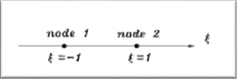
First, we discuss a one-dimensional isoparametric element to discuss the basics of isoparametric elements. Multi-dimensional elements will be discussed later. Shape functions for the isoparametric elements are given as terms of natural coordinates as seen in the following figure. Nodes are located at $\xi_=-1$ and $\xi_=1$. While the positions are arbitrary, selecting the previous values is useful, because the _natural_ coordinate system is normalized between −1 and 1.
The shape function is written as
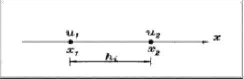
The physical linear element may be located at any position in the physical coordinate system. The element has two coordinate values $x_$ and $x_$, with two nodal variables $u_$ and $u_$.
Any point between $\xi_=-1$ and $\xi_=1$ in the _natural_ coordinate system can be mapped onto a point between $x_$ and $x_$ in the _physical_ coordinate system using the shape functions defined in Eqs. (1) and (2).
The shape functions are also used to interpolate the variable $ u $ within the element as
If the shape functions are used for geometric mapping as well as nodal variable interpolation, the element is called isoparametric element.
To compute $ \frac $, which is necessary in most of the cases to compute element matrices, we use the chain rule as
where we require $ \frac $ which is the inverse of $ \frac $. We can compute the latter from Eq.(3).
The Jacobian becomes
Substituting Eq. (6) into Eq. (5) results in
Derivatives of shape functions with respect to physical coordinate system are
where $ h_=\left(x_-x_\right) $ is the element size in the _physical_ coordinate system.
At this point, the isoparamteric element does not seem to have an advantage over the conventional element because the isoparamteric element requires more steps such as applying the chain rule and mapping. The major advantage of isoparametric elements comes when analytical integration to compute element stiffness matrices and system vectors is either complicated or impossible. This is when element shapes are not regular or differential equations are complex. Therefore, we need a numerical integration technique. Because each isoparamteric element is defined in terms of the normalized domain $\xi_=-1$ and $ \xi_=1 $, it is easier to apply any numerical integration technique.
Triangular and quadrilateral finite elements make it possible for the direct assembly of the stiffness matrices and vectors of nodal forces. The calculation of the shape functions and assembly of the stiffness matrices for quadrilateral and higher order elements are achieved with using isoparametric elements.
The construction of trial solution over a finite element must satisfy the requirements of the problem to solve the geometry of the element. Depending on the type of the problem a trial solution must be continuous, and its derivative must exist (such as a bar problem) or the trial solution and its first derivative must be continuous, and its second derivative must exist (beam problem) and so on.
The compatibility principle, thus, can be formulated as:
When the size of an element shrinks to zero, the trail function must be able to represent:
These conditions (compatibility and completeness) are sufficient to ensure that the finite element solution converges to the exact solution. However, the solutions obtained with the finite element method are only approximations to the exact solutions, therefore it is worthwhile to understand these principles to assess the accuracy or make a diagnosis of a finite element model.
Shape functions for a bilinear isoparametric element are: